AWD 3302: Project Files

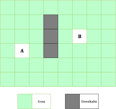
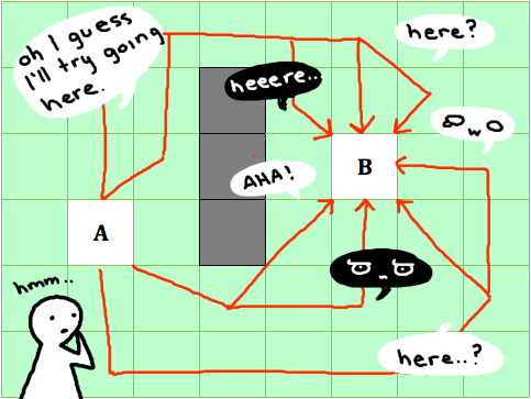
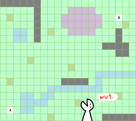
Connect The Dots: Graphs

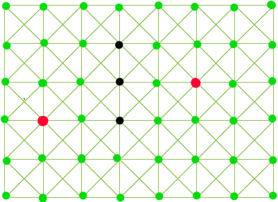
A graph is a collection of nodes or vertices, connected by edges. A square has 4 nodes and 4 edges: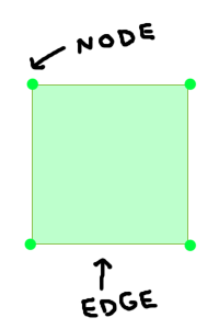

The nodes represent some sort of data, so we don’t need to depict them as points like above. Think of constellations!

Ah, but how does that relate to our problem? Well, let’s look at our map again.^[i.n.]

In this case, the nodes represent our terrain tiles, and the edges represent the connection between adjacent tiles (directly horizontal/vertical or diagonal). Throughout, I will use node and tile interchangeably, leaning towards node. The graph representing our tile map is shown below.

To further clarify, let’s look at tile A. There are 8 adjacent tiles connected to A directly. We call these tiles “neighbors” of A.

Got it? Great! We can finally move on to our three algo brothers.

Shhh, shhh, A*, it’s not your time to shine yet. We need to look at your bros first.

---

Chapter 2: Meet the Algorithms

-Bro #1: Dijkstra’s Algorithm
-Bro #2: Best-First Search Algorithm
-A* Is Born

---

Bro #1: Dijkstra’s Algorithm

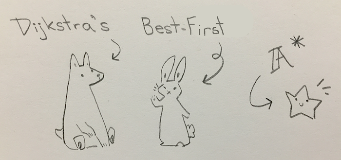
Dijkstra's Algorithm is like a dog who's slow but very thorough in his search.

It finds the shortest path from a source node to all other nodes. Each of our nodes holds some data. The main pieces of data they hold are (1) the tentative cost from the start A to the node and (2) the parent of the node (i.e. the previous node that this node came from). Notice how I say “cost” rather than distance. In a graph, we can give our edges any value; it doesn’t necessarily have to be distance between nodes. Think of if we wanted to add a body of water to the map:

If we wanted to mark the body of water as more difficult to cross than the grasslands, we can make the cost to cross it greater than that of grass. But for now, we’ll ignore any extra terrain until we meet A* for simplicity.

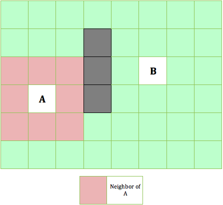
Now, if we haven’t reached the nodes yet, how do we know that information? Ah, that’s a good point. Really, we don’t know, so we will initialize all of the nodes, except A, with an infinite distance and say that they have no parent. Giving them an infinite distance may seem weird, but this ensures that we update it the first time we find a path to it (since the cost we find to it will definitely be less than infinity).

We also have a list, initially empty, that tracks the nodes we visited. To begin the algorithm, we place A on this visited list and then repeat the following steps until we run out of nodes to visit.

(1) Find an unvisited node closest to our current node
(2) Go to that node and mark it as visited. This means that we have found the shortest path from A to the current node. Thus, if the new node is our goal, we can stop the algorithm. The steps following it are to ensure that we also get the shortest path from A to its neighbors. But really, if we reached the end, we don’t care about them anymore. But if this wasn’t the goal, go on to 3)
(3) Look at all of the neighbors of this new node. If the cost of the path going from A to the neighbor in which we pass through the current node is shorter than any previous distance to the neighbor, update it with the shorter path (cost and parent). Another way to look at this is that the cost from A to the particular neighbor we’re looking at is the cost from A to the current tile + the cost of the current tile to the particular neighbor.

Eventually, we will run out of nodes to inspect and end up with a list of the shortest paths from A to all other nodes. If we find that the cost from A to a particular node is still infinity, then there is no path to between the two. Alright, that may have been a little confusing, so let me walk you through the algorithm on our map. We place A on our visited list and inspect its neighbors, marking the cost of each neighbor to A.

Additionally, we mark A as the parent of those nodes. We do this by drawing arrows from those neighbors to A.

Next, we go to the lowest cost neighbor. In this case, we have four of those (each with a value of 10)! How do we choose? Well, for Dijkstra’s, it doesn’t matter. Implementation-wise, we will probably go to the last node we discovered. What this may affect is which shortest path we end up taking if there are multiple shortest paths. Then, we inspect the neighbors of this new node.

Next, we mark place the node on the visited list and go on to inspect the other three lowest cost neighbors of A.

Nice! Covered all the 10’s. Now, you continue. What nodes haven’t been visited and have the lowest cost to A now? The diagonal nodes, so visit them and inspect their neighbors to see if going through them gives their neighbors a lower cost path to A (in this case it doesn’t).

We’re done with the 14 cost ones now, so we keep going. Eventually we’ll have something like this:

Tile B is the neighbor of our current node, so we can stop the algorithm and backtrack through the parents we tracked. The shortest path from B to A is highlighted red below (reverse it to get the path from A to B). If you trace the arrows from the other tiles, you’ll also notice that they are shortest paths from themselves to A.

And that’s it! If you got all of that, you’ve almost got A* down too, but before we go there, let’s look at Bro #2 to really get the full picture.

Bro #2: Best-First Search Algorithm

Best-First Search is like a speedy bunny who is so focuses on the end goal that he ends up ignoring potentially better paths.

Unlike Dijkstra’s, this algorithm uses a heuristic to estimate the shortest path between A and B (recall that Dijkstra’s is from A to any other node). A heuristic is a method where we use an educated “guess” to lead us to the solution.

What you did before was randomly guessing. This is using an educated guess as a guide. Think of a detective who’s searching for a criminal. If she doesn’t have anything to go off, she has to visit every district. But if she gets a good clue that the criminal is around District A, she can direct her investigation there. We can think of the heuristic as a tipoff.

In Best-First, the heuristic is the estimated cost from the current node to the end node B. There are various ways to get the heuristic value, but the most common way is with the Manhattan method. This method counts the distance traversed only horizontally and vertically to get to the end, ignoring any diagonal movement and obstacles. This distance, also called the taxicab distance, is named after the New York borough Manhattan, which is known for its grid-like streets.

Best-First trades accuracy for speed. If we have no obstacles, BFS works well. Below we go through a simple run-through of Best-First. The numbers on the tiles are the Manhattan distance from those nodes to B.

But if we end up introducing a wall, the path will resemble this:

That’s because Best-First only thinks of the distance to the end and fails to update the path prior to the wall. In this case, if the wrong lowest cost is chosen, it will keep going and disregard early nodes even if they turn out to be more optimal later. Remember choosing between lowest cost nodes didn’t matter for Dijkstra’s because he goes back to check, but it matters for Best-First because he’ll keep going towards nodes closer to the end. Anyway, that’s all you really need to know, so let’s finally meet A*!

A* Is Born

A* is a fusion of Dijkstra’s and Best-First.

He takes into account both the cost from the start to the current node and the cost from the current node to the end.

F = G + H

Where

G = cost from the start to the current node

H = estimated cost from the current node to the end

G will be calculated the same way as in Dijkstra’s while H will be calculated the same way as in Best-First with the Manhattan distance. Remember, we say H, the heuristic value, is an estimate because there are many things that it doesn’t take into account, like obstacles. We’ll go back to the steps outlined for Dijkstra’s, except we will update it so that we inspect the nodes with the lowest F cost first.

To begin the algorithm, we place A on the visited list and then repeat the following steps until we run out of nodes to visit:

(1) Find an unvisited node with the lowest F cost.
(2) Go to that node and mark it as visited. If the new node is our goal, stop the algorithm; else, go on to 3)
(3) Look at all of the neighbors of this new node. If the G cost of the path going from A to the neighbor in which we pass through the current node is shorter than any previous distance to the neighbor, update it with the shorter path (cost and parent).

Alright, let’s go through our map now.

Now, observe below. When we make the top 50 value node our current node, we update the neighbor above it. That’s because the path from A to that node of 70 is shorter than the path from A to that node if we were to come from the 44-value node.

Nice looking path! Great job A*! Let’s dig a bit deeper though.

---

Chapter 3: More on A*

-Weighted Tiles
-Suboptimal Path
-Comparisons

---

Weighted Tiles

Let’s say we decide to add a river to our map. We can cross it, but it takes a lot of effort to, so we decide to add an extra value of 30 on top of the normal 10 for going horizontal or 14 to go diagonal. This will make the algorithm skirt around the river to find a less costly way to get to B.

Suboptimal Path

Hey, A*! You’re doing so well! What if we add to this river? Let’s go back to where it’ll change. At some point, we’ll get here:

And after we run through completely, we’ll get this:

That gives us this path:

Pretty nice! I think tha- WAIT A MINUTE. THAT’S A SUBOPTIMAL PATH. The optimal one is this:

Alright, back up. What just happened? Well, A* is taking after his brother First-Best. At some point we have to choose a lowest cost node (refer back to the image above where the lowest cost node of value 78 is chosen). The estimates place those nodes on the same value, but if we look closely, we can see that the G value of the top value 78 node should be a bit less (because we can get to B through diagonals). This may happen depending on how estimates and lowest cost nodes are chosen during implementation, so just be aware!

Comparison

Besides that occasional mishap, which can be fixed with different implementations, A* is a good combination of Dijkstra’s and Best-First. Let’s do a comparison of the algorithms. Below is a run-through of the three algorithms on a large map. It’s important to note that diagonals are not counted as neighbors here, so we can only move directly horizontally or vertically. Dijkstra’s spends more time exploring the map and gets the correct shortest path. Meanwhile, Best-First, doesn’t spend as much time exploring but also doesn’t find the shortest path. Instead, he bumps into the wall before correcting himself. Lastly, A* spends only a bit of time exploring and finds the correct path.

---

End: Expanding Horizons

---

There’s quite a lot you can do with pathfinding! In this post, I showed you three pathfinding algorithms: Dijkstra’s, Best-First, and A*. We focused on A* because it combines the efficiency of Dijkstra’s with the speed of Best-First. A* is the most popular pathfinding algorithm in game development. If you’re interested in learning more, start checking out how weights can affect your units’ movements. For example, you can add them to particular terrain tiles like we did above with the river or subtract them from tiles acting as stairs/teleporters, which take you closer to the target. Also, your tiles don’t have to be squares. You can use hexagonal shapes, and the algorithms still work the same. That actually makes the math easier since the distance to each neighbor is equal. Additionally, it’ll be good to consider movement restrictions, such as those dealing with cutting corners or units that takes^[i.n.] up more than one tile space. I recommend checking out the sources below too. RedBlobGames^[i.n.] provides great interactive visuals on the algorithms. The author doesn’t use diagonal neighbors in his examples (so only a max of four neighbors for a node), but don’t be confused! The algorithms work the same way!

That’s all for now! Happy pathfinding!